How you can train AI to convert design mockups into HTML and CSS

Within three years, deep learning will change front-end development. It will increase prototyping speed and lower the barrier for building software.

The field took off last year when Tony Beltramelli introduced the pix2code paper and Airbnb launched sketch2code.

Currently, the largest barrier to automating front-end development is computing power. However, we can use current deep learning algorithms, along with synthesized training data, to start exploring artificial front-end automation right now.

In this post, we’ll teach a neural network how to code a basic HTML and CSS website based on a picture of a design mockup using deep-learning platform FloydHub. Here’s a quick overview of the process:

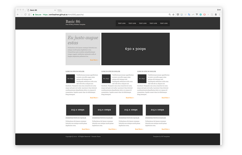
1) Give a design image to the trained neural network

2) The neural network converts the image into HTML markup

3) Rendered output

We’ll build the neural network in three iterations.

First, we’ll make a bare minimum version to get a hang of the moving parts. The second version, HTML, will focus on automating all the steps and explaining the neural network layers. In the final version, Bootstrap, we’ll create a model that can generalize and explore the LSTM layer.

All the code is prepared on Github and FloydHub in Jupyter notebooks. All the FloydHub notebooks are inside the floydhub directory and the local equivalents are under local.

The models are based on Beltramelli‘s pix2code paper and Jason Brownlee’s image caption tutorials. The code is written in Python and Keras, a framework on top of TensorFlow.

If you’re new to deep learning, I’d recommend getting a feel for Python, backpropagation, and convolutional neural networks. My three earlier posts on FloydHub’s blog will get you started:

• My First Weekend Of Deep Learning
• Coding The History Of Deep Learning
• Colorizing B&W Photos with Neural Networks

Core Logic

Let’s recap our goal. We want to build a neural network that will generate HTML/CSS markup that corresponds to a screenshot.

When you train the neural network, you give it several screenshots with matching HTML.

It learns by predicting all the matching HTML markup tags one by one. When it predicts the next markup tag, it receives the screenshot as well as all the correct markup tags until that point.

Here is a simple training data example in a Google Sheet.

Creating a model that predicts word by word is the most common approach today. There are other approaches, but that’s the method we’ll use throughout this tutorial.

Notice that for each prediction it gets the same screenshot. So if it has to predict 20 words, it will get the same design mockup twenty times. For now, don’t worry about how the neural network works. Focus on grasping the input and output of the neural network.

Let’s focus on the previous markup. Say we train the network to predict the sentence “I can code.” When it receives “I,” then it predicts “can.” Next time it will receive “I can” and predict “code.” It receives all the previous words and only has to predict the next word.

The neural network creates features from the data. The network builds features to link the input data with the output data. It has to create representations to understand what is in each screenshot, the HTML syntax, that it has predicted. This builds the knowledge to predict the next tag.

When you want to use the trained model for real-world usage, it’s similar to when you train the model. The text is generated one by one with the same screenshot each time. Instead of feeding it with the correct HTML tags, it receives the markup it has generated so far. Then, it predicts the next markup tag. The prediction is initiated with a “start tag” and stops when it predicts an “end tag” or reaches a max limit. Here’s another example in a Google Sheet.

“Hello World” Version

Let’s build a “hello world” version. We’ll feed a neural network a screenshot with a website displaying “Hello World!” and teach it to generate the markup.

First, the neural network maps the design mockup into a list of pixel values. From 0–255 in three channels — red, blue, and green.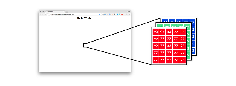

To represent the markup in a way that the neural network understands, I use one hot encoding. Thus, the sentence “I can code” could be mapped like the below.

In the above graphic, we include the start and end tag. These tags are cues for when the network starts its predictions and when to stop.

For the input data, we will use sentences, starting with the first word and then adding each word one by one. The output data is always one word.

Sentences follow the same logic as words. They also need the same input length. Instead of being capped by the vocabulary, they are bound by maximum sentence length. If it’s shorter than the maximum length, you fill it up with empty words, a word with just zeros.

As you see, words are printed from right to left. This forces each word to change position for each training round. This allows the model to learn the sequence instead of memorizing the position of each word.

In the below graphic there are four predictions. Each row is one prediction. To the left are the images represented in their three color channels: red, green and blue and the previous words. Outside of the brackets are the predictions one by one, ending with a red square to mark the end.

Here is a link to the Jupyter notebook with the Hello World code snippet.

In the hello world version, we use three tokens: start, <HTML><center><H1>Hello World!</H1></center></HTML> and end. A token can be anything. It can be a character, word, or sentence. Character versions require a smaller vocabulary but constrain the neural network. Word level tokens tend to perform best.

Output

• 10 epochs: start start start
• 100 epochs: start <HTML><center><H1>Hello World!</H1></center></HTML> <HTML><center><H1>Hello World!</H1></center></HTML>
• 300 epochs: start <HTML><center><H1>Hello World!</H1></center></HTML> end

Mistakes I made:

• Build the first working version before gathering the data. Early on in this project, I managed to get a copy of an old archive of the Geocities hosting website. It had 38 million websites. Blinded by the potential, I ignored the huge workload that would be required to reduce the 100K-sized vocabulary.
• Dealing with a terabyte worth of data requires good hardware or a lot of patience. After having my mac run into several problems I ended up using a powerful remote server. Expect to rent a rig with 8 modern CPU cores and a 1GPS internet connection to have a decent workflow.
• Nothing made sense until I understood the input and output data.The input, X, is one screenshot and the previous markup tags. The output, Y, is the next markup tag. When I got this, it became easier to understand everything between them. It also became easier to experiment with different architectures.
• Be aware of the rabbit holes. Because this project intersects with a lot of fields in deep learning, I got stuck in plenty of rabbit holes along the way. I spent a week programming RNNs from scratch, got too fascinated by embedding vector spaces, and was seduced by exotic implementations.
• Picture-to-code networks are image caption models in disguise. Even when I learned this, I still ignored many of the image caption papers, simply because they were less cool. Once I got some perspective, I accelerated my learning of the problem space.

Running the code on FloydHub

FloydHub is a training platform for deep learning. I came across them when I first started learning deep learning and I’ve used them since for training and managing my deep learning experiments. You can install it and run your first model within 10 minutes. It’s hands down the best option to run models on cloud GPUs.

If you are new to FloydHub, do their 2-min installation or my 5-minute walkthrough.

Clone the repository

git clone https://github.com/emilwallner/Screenshot-to-code-in-Keras.git

Login and initiate FloydHub command-line-tool

cd Screenshot-to-code-in-Keras
floyd login
floyd init s2c

Run a Jupyter notebook on a FloydHub cloud GPU machine:

floyd run --gpu --env tensorflow-1.4 --data emilwallner/datasets/imagetocode/2:data --mode jupyter

All the notebooks are prepared inside the FloydHub directory. The local equivalents are under local. Once it’s running, you can find the first notebook here: floydhub/Helloworld/helloworld.ipynb .

If you want more detailed instructions and an explanation for the flags, check my earlier post.

HTML Version

In this version, we’ll automate many of the steps from the Hello World model. This section will focus on creating a scalable implementation and the moving pieces in the neural network.

This version will not be able to predict HTML from random websites, but it’s still a great setup to explore the dynamics of the problem.

Overview

If we expand the components of the previous graphic it looks like this.

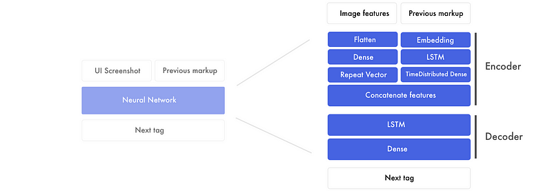
There are two major sections. First, the encoder. This is where we create image features and previous markup features. Features are the building blocks that the network creates to connect the design mockups with the markup. At the end of the encoder, we glue the image features to each word in the previous markup.

The decoder then takes the combined design and markup feature and creates a next tag feature. This feature is run through a fully connected neural network to predict the next tag.

Design mockup features

Since we need to insert one screenshot for each word, this becomes a bottleneck when training the network (example). Instead of using the images, we extract the information we need to generate the markup.

The information is encoded into image features. This is done by using an already pre-trained convolutional neural network (CNN). The model is pre-trained on Imagenet.

We extract the features from the layer before the final classification.

We end up with 1536 eight by eight-pixel images known as features. Although they are hard to understand for us, a neural network can extract the objects and position of the elements from these features.

Markup features

In the hello world version, we used a one-hot encoding to represent the markup. In this version, we’ll use a word embedding for the input and keep the one-hot encoding for the output.

The way we structure each sentence stays the same, but how we map each token is changed. One-hot encoding treats each word as an isolated unit. Instead, we convert each word in the input data to lists of digits. These represent the relationship between the markup tags.

The dimension of this word embedding is eight but often varies between 50–500 depending on the size of the vocabulary.

The eight digits for each word are weights similar to a vanilla neural network. They are tuned to map how the words relate to each other (Mikolov et al., 2013).

This is how we start developing markup features. Features are what the neural network develops to link the input data with the output data. For now, don’t worry about what they are, we’ll dig deeper into this in the next section.

The Encoder

We’ll take the word embeddings and run them through an LSTM and return a sequence of markup features. These are run through a Time distributed dense layer — think of it as a dense layer with multiple inputs and outputs.

In parallel, the image features are first flattened. Regardless of how the digits were structured, they are transformed into one large list of numbers. Then we apply a dense layer on this layer to form a high-level feature. These image features are then concatenated to the markup features.

This can be hard to wrap your mind around — so let’s break it down.

Markup features

Here we run the word embeddings through the LSTM layer. In this graphic, all the sentences are padded to reach the maximum size of three tokens.

To mix signals and find higher-level patterns, we apply a TimeDistributed dense layer to the markup features. TimeDistributed dense is the same as a dense layer, but with multiple inputs and outputs.

Image features

In parallel, we prepare the images. We take all the mini image features and transform them into one long list. The information is not changed, just reorganized.

Again, to mix signals and extract higher-level notions, we apply a dense layer. Since we are only dealing with one input value, we can use a normal dense layer. To connect the image features to the markup features, we copy the image features.

In this case, we have three markup features. Thus, we end up with an equal amount of image features and markup features.

Concatenating the image and markup features

All the sentences are padded to create three markup features. Since we have prepared the image features, we can now add one image feature for each markup feature.

After sticking one image feature to each markup feature, we end up with three image-markup features. This is the input we feed into the decoder.

The Decoder

Here we use the combined image-markup features to predict the next tag.

In the below example, we use three image-markup feature pairs and output one next tag feature.

Note that the LSTM layer has the sequence set to false. Instead of returning the length of the input sequence, it only predicts one feature. In our case, it’s a feature for the next tag. It contains the information for the final prediction.

The final prediction

The dense layer works like a traditional feedforward neural network. It connects the 512 digits in the next tag feature with the 4 final predictions. Say we have 4 words in our vocabulary: start, hello, world, and end.

The vocabulary prediction could be [0.1, 0.1, 0.1, 0.7]. The softmax activation in the dense layer distributes a probability from 0–1, with the sum of all predictions equal to 1. In this case, it predicts that the 4th word is the next tag. Then you translate the one-hot encoding [0, 0, 0, 1] into the mapped value, say “end”.

Here is a link to the Jupyter notebook with the HTML code snippet.

Output

Links to generated websites

• 250 epochs
• 350 epochs
• 450 epochs
• 550 epochs

If you can’t see anything when you click these links, you can right click and click on “View Page Source.” Here is the original website for reference.

Mistakes I made:

• LSTMs are a lot heavier for my cognition compared to CNNs. When I unrolled all the LSTMs, they became easier to understand. Fast.ai’s video on RNNs was super useful. Also, focus on the input and output features before you try understanding how they work.
• Building a vocabulary from the ground up is a lot easier than narrowing down a huge vocabulary. This includes everything from fonts, div sizes, and hex colors to variable names and normal words.
• Most of the libraries are created to parse text documents and not code. In documents, everything is separated by a space, but in code, you need custom parsing.
• You can extract features with a model that’s trained on Imagenet.This might seem counterintuitive since Imagenet has few web images. However, the loss is 30% higher compared to a pix2code model, which is trained from scratch. It’d be interesting to use a pre-train inception-resnet type of model based on web screenshots.

Bootstrap version

In our final version, we’ll use a dataset of generated bootstrap websites from the pix2code paper. By using Twitter’s bootstrap, we can combine HTML and CSS and decrease the size of the vocabulary.

We’ll enable it to generate the markup for a screenshot it has not seen before. We’ll also dig into how it builds knowledge about the screenshot and markup.

Instead of training it on the bootstrap markup, we’ll use 17 simplified tokens that we then translate into HTML and CSS. The dataset includes 1500 test screenshots and 250 validation images. For each screenshot there are on average 65 tokens, resulting in 96925 training examples.

By tweaking the model in the pix2code paper, the model can predict the web components with 97% accuracy (BLEU 4-ngram greedy search, more on this later).

An end-to-end approach

Extracting features from pre-trained models works well in image captioning models. But after a few experiments, I realized that pix2code’s end-to-end approach works better for this problem. The pre-trained models have not been trained on web data and are customized for classification.

In this model, we replace the pre-trained image features with a light convolutional neural network. Instead of using max-pooling to increase information density, we increase the strides. This maintains the position and the color of the front-end elements.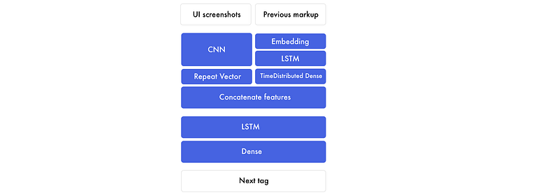

There are two core models that enable this: convolutional neural networks (CNN) and recurrent neural networks (RNN). The most common recurrent neural network is long-short-term memory (LSTM), so that’s what I’ll refer to.

There are plenty of great CNN tutorials, and I covered them in my previous article. Here, I’ll focus on the LSTMs.

Understanding timesteps in LSTMs

One of the harder things to grasp about LSTMs is timesteps. A vanilla neural network can be thought of as two timesteps. If you give it “Hello,” it predicts “World.” But it would struggle to predict more timesteps. In the below example, the input has four timesteps, one for each word.

LSTMs are made for input with timesteps. It’s a neural network customized for information in order. If you unroll our model it looks like this. For each downward step, you keep the same weights. You apply one set of weights to the previous output and another set to the new input.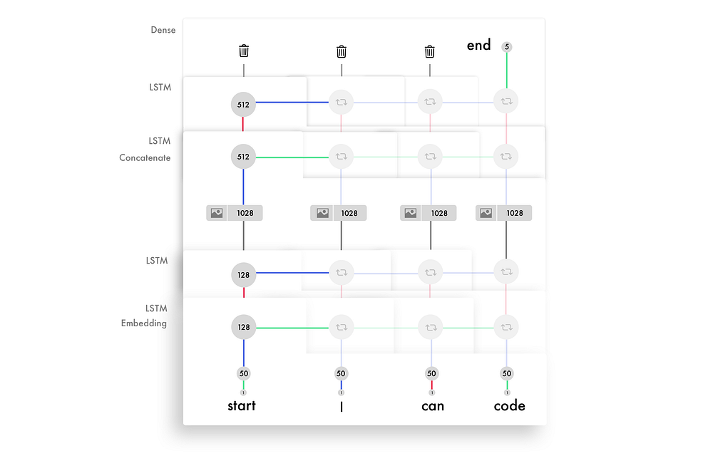

The weighted input and output are concatenated and added together with an activation. This is the output for that timestep. Since we reuse the weights, they draw information from several inputs and build knowledge of the sequence.

Here is a simplified version of the process for each timestep in an LSTM.

To get a feel for this logic, I’d recommend building an RNN from scratch with Andrew Trask’s brilliant tutorial.

Understanding the units in LSTM layers

The number of units in each LSTM layer determines it’s ability to memorize. This also corresponds to the size of each output feature. Again, a feature is a long list of numbers used to transfer information between layers.

Each unit in the LSTM layer learns to keep track of different aspects of the syntax. Below is a visualization of a unit that keeps tracks of the information in the row div. This is the simplified markup we are using to train the bootstrap model.

Each LSTM unit maintains a cell state. Think of the cell state as the memory. The weights and activations are used to modify the state in different ways. This enables the LSTM layers to fine-tune which information to keep and discard for each input.

In addition to passing through an output feature for each input, it also forwards the cell states, one value for each unit in the LSTM. To get a feel for how the components within the LSTM interact, I recommend Colah’s tutorial, Jayasiri’s Numpy implementation, and Karphay’s lecture and write-up.

Here is a link to the Jupyter notebook with the Bootstrap code snippet.

Test accuracy

It’s tricky to find a fair way to measure the accuracy. Say you compare word by word. If your prediction is one word out of sync, you might have 0% accuracy. If you remove one word which syncs the prediction, you might end up with 99/100.

I used the BLEU score, best practice in machine translating and image captioning models. It breaks the sentence into four n-grams, from 1–4 word sequences. In the below prediction “cat” is supposed to be “code.”

To get the final score, you multiply each score with 25%, (4/5) * 0.25 + (2/4) * 0.25 + (1/3) * 0.25 + (0/2) * 0.25 = 0.2 + 0.125 + 0.083 + 0 = 0.408 . The sum is then multiplied with a sentence length penalty. Since the length is correct in our example, it becomes our final score.

You could increase the number of n-grams to make it harder. A four n-gram model is the model that best corresponds to human translations. I’d recommend running a few examples with the below code and reading the wiki page.

Here is a link to the Jupyter notebook with the rest of the Bootstrap code snippet.

Output

Links to sample output

• Generated website 1 — Original 1
• Generated website 2 — Original 2
• Generated website 3 — Original 3
• Generated website 4 — Original 4
• Generated website 5 — Original 5

Mistakes I made:

• Understand the weakness of the models instead of testing random models. First, I applied random things such as batch normalization and bidirectional networks and tried implementing attention. After looking at the test data and seeing that it could not predict color and position with high accuracy, I realized there was a weakness in the CNN. This led me to replace maxpooling with increased strides. The validation loss went from 0.12 to 0.02 and increased the BLEU score from 85% to 97%.
• Only use pre-trained models if they are relevant. Given the small dataset, I thought that a pre-trained image model would improve the performance. From my experiments, and end-to-end model is slower to train and requires more memory, but is 30% more accurate.
• Plan for slight variance when you run your model on a remote server.On my mac, it reads the files in alphabetic order. However, on the server, it was randomly located. This created a mismatch between the screenshots and the code. It still converged, but the validation data was 50% worse than when I fixed it.
• Make sure you understand library functions. Include space for the empty token in your vocabulary. When I didn’t add it, it did not include one of the tokens. I only noticed it after looking at the final output several times and noticing that it never predicted a “single” token. After a quick check, I realized it wasn’t even in the vocabulary. Also, use the same order in the vocabulary for training and testing.
• Use lighter models when experimenting. Using GRUs instead of LSTMs reduced each epoch cycle by 30%, and did not have a large effect on the performance.

Next steps

Front-end development is an ideal space to apply deep learning. It’s easy to generate data, and the current deep learning algorithms can map most of the logic.

One of the most exciting areas is applying attention to LSTMs. This will not just improve the accuracy, but enable us to visualize where the CNN puts its focus as it generates the markup.

Attention is also key for communicating between markup, stylesheets, scripts and eventually the backend. Attention layers can keep track of variables, enabling the network to communicate between programming languages.

But in the near feature, the biggest impact will come from building a scalable way to synthesize data. Then you can add fonts, colors, words, and animations step-by-step.

So far, most progress is happening in taking sketches and turning them into template apps. In less then two years, we’ll be able to draw an app on paper and have the corresponding front-end in less than a second. There are already two working prototypes built by Airbnb’s design team and Uizard.

Here are some experiments to get started.

Experiments

Getting started

• Run all the models
• Try different hyper parameters
• Test a different CNN architecture
• Add Bidirectional LSTM models
• Implement the model with a different dataset. (You can easily mount this dataset in your FloydHub jobs with this flag --data emilwallner/datasets/100k-html:data)

Further experiments

• Creating a solid random app/web generator with the corresponding syntax.
• Data for a sketch to app model. Auto-convert the app/web screenshots into sketches and use a GAN to create variety.
• Apply an attention layer to visualize the focus on the image for each prediction, similar to this model.
• Create a framework for a modular approach. Say, having encoder models for fonts, one for color, another for layout and combine them with one decoder. A good start could be solid image features.
• Feed the network simple HTML components and teach it to generate animations using CSS. It would be fascinating to have an attention approach and visualize the focus on both input sources.

Huge thanks to Tony Beltramelli and Jon Gold for their research and ideas, and for answering questions. Thanks to Jason Brownlee for his stellar Keras tutorials (I included a few snippets from his tutorial in the core Keras implementation), and Beltramelli for providing the data. Also thanks to Qingping Hou, Charlie Harrington, Sai Soundararaj, Jannes Klaas, Claudio Cabral, Alain Demenet and Dylan Djian for reading drafts of this.

About Emil Wallner

This the fourth part of a multi-part blog series from Emil as he learns deep learning. Emil has spent a decade exploring human learning. He’s worked for Oxford’s business school, invested in education startups, and built an education technology business. Last year, he enrolled at Ecole 42 to apply his knowledge of human learning to machine learning.

If you build something or get stuck, ping me below or on Twitter: emilwallner. I’d love to see what you are building.