(AI) and computer science that enables automated systems to see, i.e. to process images and video in a human-like manner to detect and identify objects or regions of importance, predict an outcome or even alter the image to a desired format [1]. Most popular use cases in the CV domain include automated perception for autonomous drive, augmented and virtual realities (AR, VR) for simulations, games, glasses, reality, and fashion or beauty-oriented e-commerce.
Medical image (MI) processing on the other hand involves much more detailed analysis of medical images that are typically grayscale such as MRI, CT, or X-ray images for automated pathology detection, a task that requires a trained specialist’s eye for detection. Most popular use cases in the MI domain include automated pathology labeling, localization, association with treatment or prognostics, and personalized medicine.
Prior to the advent of deep learning methods, 2D signal processing solutions such as image filtering, wavelet transforms, image registration, followed by classification models [2–3] were heavily applied for solution frameworks. Signal processing solutions still continue to be the top choice for model baselining owing to their low latency and high generalizability across data sets.
However, deep learning solutions and frameworks have emerged as a new favorite owing to the end-to-end nature that eliminates the need for feature engineering, feature selection and output thresholding altogether. In this tutorial, we will review “Top 10” project choices for beginners in the fields of CV and MI and provide examples with data and starter code to aid self-paced learning.
CV and MI solution frameworks can be analyzed in three segments: Data, Process, and Outcomes [4]. It is important to always visualize the data required for such solution frameworks to have the format “{X,Y}”, where X represents the image/video data and Y represents the data target or labels. While naturally occurring unlabelled images and video sequences (X) can be plentiful, acquiring accurate labels (Y) can be an expensive process. With the advent of several data annotation platforms such as [5–7], images and videos can be labeled for each use case.
Since deep learning models typically rely on large volumes of annotated data to automatically learn features for subsequent detection tasks, the CV and MI domains often suffer from the “small data challenge”, wherein the number of samples available for training a machine learning model is several orders lesser than the number of model parameters.
The “small data challenge” if unaddressed can lead to overfit or underfit models that may not generalize to new unseen test data sets. Thus, the process of designing a solution framework for CV and MI domains must always include model complexity constraints, wherein models with fewer parameters are typically preferred to prevent model underfitting.
Finally, the solution framework outcomes are analyzed both qualitatively through visualization solutions and quantitatively in terms of well-known metrics such as precision, recall, accuracy, and F1 or Dice coefficients [8–9].
The projects listed below present a variety in difficulty levels (difficulty levels Easy, Medium, Hard) with respect to data pre-processing and model building. Also, these projects represent a variety of use cases that are currently prevailing in the research and engineering communities. The projects are defined in terms of the: Goal, Methods, and Results.
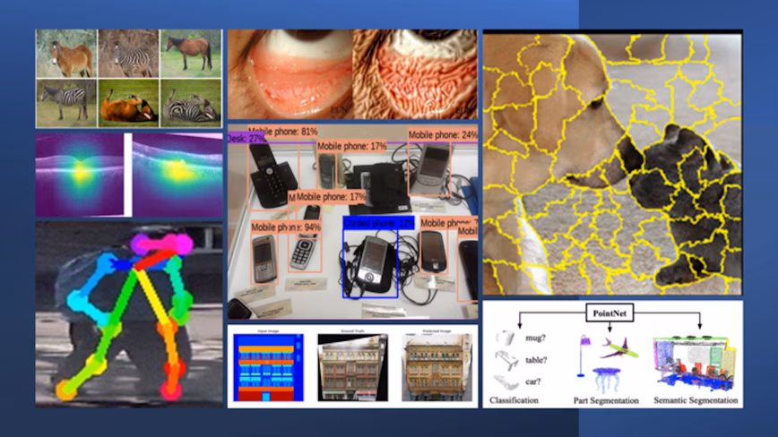
Project 1: MNIST and Fashion MNIST for Image Classification (Level: Easy)
Goal: To process images (X) of size [28×28] pixels and classify them into one of the 10 output categories (Y). For the MNIST data set, the input images are handwritten digits in the range 0 to 9 [10]. The training and test data sets contain 60,000 and 10,000 labeled images, respectively. Inspired by the handwritten digit recognition problem, another data set called the Fashion MNIST data set was launched [11] where the goal is to classify images (of size [28×28]) into clothing categories as shown in Fig. 1.
Methods: When the input image is small ([28×28] pixels) and images are grayscale, convolutional neural network (CNN) models, where the number of convolutional layers can vary from single to several layers are suitable classification models. An example of MNIST classification model build using Keras is presented in the colab file:
Another example of classification on the Fashion MNIST data set is shown in:
In both instances, the key parameters to tune include the number of layers, dropout, optimizer (Adaptive optimizers preferred), learning rate, and kernel size as seen in the code below. Since this is a multi-class problem, the ‘softmax’ activation function is used in the final layer to ensure only 1 output neuron gets weighted more than the others.
Results: As the number of convolutional layers increases from 1–10, the classification accuracy is found to increase as well. The MNIST data set is well studied in literature with test accuracies in the range of 96–99%. For the Fashion MNIST data set, test accuracies are typically in the range 90–96%. An example of visualization of the MNIST classification outcome using CNN models is shown in Fig 2 below (See visualization at front end here).
Project 2: Pathology Classification for Medical Images (Level: Easy)
Goal: To classify medical images (acquired using Optical Coherence Tomography, OCT) as Normal, Diabetic Macular Edema (DME), Drusen, choroidal neovascularization (CNV) as shown in [12]. The data set contains about 84,000 training images and about 1,000 test images with labels and each image has a width of 800 to 1,000 pixels as shown in Fig 2.
Methods: Deep CNN models such as Resnet and CapsuleNet [12] have been applied to classify this data set. The data needs to be resized to [512×512] or [256×256] to be fed to standard classification models. Since medical images have lesser variations in object categories per image frame when compared to non-medical outdoor and indoor images, the number of medical images required to train large CNN models is found to be significantly lesser than the number of non-medical images.
The work in [12] and the OCT code base demonstrates retraining the ResNet layer for transfer learning and classification of test images. The parameters to be tuned here include optimizer, learning rate, size of input images, and number of dense layers at the end of the ResNet layer.
Results: For the ResNet model test accuracy can vary between 94–99% by varying the number of training images as shown in [12]. Fig 3. qualitatively demonstrates the performance of the classification model.
These visualizations are produced using the Gradcam library that combines the CNN layer activations onto the original image to understand the regions of interest, or automatically detected features of importance, for the classification task. Usage of Gradcam using the tf_explain library is shown below.
Project 3: AI Explainability for Multi-label Image Classification (Level: Easy)
Goal: CNN models enable end-to-end delivery, which means there is no need to engineer and rank features for classification and the model outcome is the desired process outcome. However, it is often important to visualize and explain CNN model performances as shown in later parts of Project 2.
Some well-known visualization and explainability libraries are tf_explain and Local Interpretable Model-Agnostic Explanations (LIME). In this project, the goal is to achieve multi-label classification and explain what the CNN model is seeing as features to classify images in a particular way. In this case, we consider a multi-label scenario wherein one image can contain multiple objects, for example cat and a dog in Colab for LIME.
Here, the input is images with cat and dog in it and the goal is to identify which regions correspond to a cat or dog respectively.
Method: In this project, each image is subjected to super-pixel segmentation that divides the image into several sub-regions with similar pixel color and texture characteristics. The number of divided sub-regions can be manually provided as a parameter. Next, the InceptionV3 model is invoked to assign a probability to each superpixel sub-region to belong to one of the 1000 classes that InceptionV3 is originally trained on. Finally, the object probabilities are used as weights to fit a regression model that explains the ROIs corresponding to each class as shown in Fig. 4 and code below.
Results: Using the proposed method, ROIs in most non-medical images should be explainable. Qualitative assessment and explainability as shown here are specifically useful in corner cases, or in situations where the model misclassified or missed objects of interest. In such situations, explaining what the CNN model is looking at and boosting ROIs accordingly to correct overall classification performances can help significantly reduce data-induced biases.
Project 4: Transfer learning for 2D Bounding box detection on new objects (Level: Medium)
Goal: The next step after image classification is the detection of objects of interest by placing bounding boxes around them. This is a significant problem in the autonomous drive domain to accurately identify moving objects such as cars and pedestrians from static objects such as roadblocks, street signs, trees, and buildings.
The major difference between this project and the prior projects is the format of data. Here, labels Y are typically in the form of [x,y,w,h] per object of interest, where (x,y) typically represent the top left corner of the bounding box and w and h correspond to the width and height of the output bounding box. In this project, the goal is to leverage a pre-trained classifier for its feature extraction capabilities and then to retrain it on a small set of images to create a tight bounding box around a new object.
Method: In the code Bounding Box colab, we can extend a pre-trained object detector such as a single shot detector (SSD) with Resnet50 skip connections and feature pyramid network backbone, that is pre-trained for object detection on the MS-COCO dataset [13] to detect a completely unseen new object category, a rubber duck in this case.
In this transfer learning setup, the already learned weights from early layers of the object detector are useful to extract local structural and textural information from images and only the final classifier layer requires retraining for the new object class. This enables retraining the object detector for a new class, such as a rubber duck in this use case, using as few as 5–15 images of the new object. The parameters to be tuned include optimizer, learning rate, input image size, and number of neurons in the final classifier layer.
Results: One major difference between object detectors and the prior CNN-based classifier models shown above is an additional output metric called Intersection over Union (IoU) [11] that measures the extent of overlap between the actual bounding box and the predicted bounding box. Additionally, an object detector model typically consists of a classifier (that predicts the object class) and a bounding box regressor that predicts the dimensions of the bounding box around the object. An example of the Google API for object detection on a new unseen image is shown in Fig. 5 and code below.
Extensions of the 2D bounding box detector to 3D bounding boxes specifically for autonomous drive are shown in these projects.
Project 5: Personalized Medicine and Explainability (Level: Medium)
Goal: In this project, the goal is to automatically segment ROIs from multiple pathology sites to classify the extent of anemia-like pallor in a patient and track the pallor over time [13]. The two major differences in this project from the previous ones is that: 1) pallor needs to be detected across multiple image sites such as conjunctiva (under eye) and tongue to predict a single label as shown in Fig. 6, 2) ROIs corresponding to pallor need to be displayed and tracked over time.
Methods: For this project, feature-based models and CNN-based classifiers are applied with heavy data augmentation using the Imagedata generator in Keras. To fuse the outcomes from multiple pathology sites, early, mid and late fusion can be applied.
The work in [13] applies late fusion wherein the layer before the classifier, which is considered to be the optimal feature representation of the image, is used to fuse features across multiple pathological sites. Finally, the Deepdream algorithm, as shown in the Deepdream Colab, is applied to the original eye and tongue images to visualize the ROIs and explain the extent of pathology. The parameters to tune in this project include the parameters from Project 2 along with additive gradient factor for the Deepdream visualizations.
Results: The data for this work is available for benchmarking. Using the Deepdream algorithm the visualizations are shown in Fig. 7, where, we observe a higher concentration of features corresponding to pallor in the blood vessels under-eye than anywhere else in the eye. Similarly, we observe differences in features between the inner and outer segments of the tongue. These assessments are useful to create a personalized pathology tracking system for patients with anemia.
Project 6: Point cloud segmentation for object detection. (Level: Hard)
Goal: In this project, the input is a stream of point clouds, i.e., the output from Lidar sensors that provide depth resolution. The primary difference between Lidar point clouds and an image is that point clouds provide 3D resolution, so each voxel (3D equivalent of pixel) represents the location of an object from the Lidar source and height of the object relative to the Lidar source. The main challenges posed by point cloud data models are i) model computational complexity if 3D convolutions are used and ii) object transformation invariance, which means a rotated object should be detected as the object itself as shown in [13].
Method: The data set for this project is the ModelNet40 shape classification benchmark that contains over 12,000, 3D models from 40 object classes. Each object is sub-sampled to extract a fixed number of points followed by augmentation to cater to multiple transformations in shape. Next 1D convolutions are used to learn the shapeness features using the Pytorch library in the Pointnet colab as shown below.
Results: The outcome of the model can be summarized using Fig. 8 below. Up to 89% training accuracy for object classification can be achieved by this method that can also be extended to 3D semantic segmentation. Extensions to this work can be useful for 3D bounding box detection for autonomous drive use cases.
Project 7: Image semantic segmentation using U-net for binary and multi-class. (Medium)
Goal: The CNN models so far have been applied to automatically learn features that can then be used for classification. This process is known as feature encoding. As a next step, we apply a decoder unit with similar structure as the encoder to enable generation of an output image. This combination of encoder-decoder pair enables the input and output to have similar dimensions, i.e. input is an image and output is also an image.
Methods: The encoder-decoder combination with residual skip connections is popularly known as the U-net [15]. For binary and multi-class problems, the data has to be formatted such that if X (input image) has dimensions [m x m] pixels, Y has dimensions [m x m x d], where ‘d’ is the number of classes to be predicted. The parameters to tune include optimizer, learning rate, and depth of the U-net model as shown in [15] and Fig. 9 below (source here).
Results: The U-net model can learn to generate binary and multi-class semantic maps from large and small data sets [16–17], but it is found to be sensitive to data imbalance. Thus, selecting the right training data set is significantly important for optimal outcomes. Other extensions to this work would include DenseNet connections to the model, or other encoder-decoder networks such as MobileNet or Exception networks [17].
Project 8: Machine Translation for Posture and Intention Classification (Level: Hard)
Goal: Automated detection of posture or gesture often includes keypoint identification (such as identification of the skeletal structure) in videos that can lead to identification of posture (standing, walking, moving) or intention for pedestrians (crossing road, not crossing), etc. [18–19], as shown in Fig. 10 below. For this category of problems, keyframe information from multiple subsequent video frames is processed collectively to generate pose/intention-related predictions.
Methods: For this project, the class of models applied are known as “Sequence To Sequence” models, where a sequence of image frames from a video are processed to predict pedestrian intention if they are going to cross the street or not. The process initiates with a 2D bounding box detector to isolate pedestrians, followed by real time-tracking to track the same bounding box across frames.
Finally, features from the tracked bounding boxes and skeletal features are used to train a DenseNet model that predicts if a pedestrian will move in front of the moving car or not. The parameters to be tuned include bounding box detector parameters from Project 4, number of layers of the Densenet model, and the number of skeletal points fitted per pedestrian gesture. Higher the number of skeletal points, higher computational complexity is incurred.
Results: Qualitative results for the method above are shown in Fig. 11 below, where a red box indicates pedestrians that will cross the street vs. green boxes indicate pedestrians that will not cross paths with the incoming vehicle. The work in [18–19] and the Colab files can be used to test the composite models that use features inside the bounding boxes and skeletal features as an early fusion setup on any new data set to generate posture-related predictions from a sequence of image frames.
Project 9: Generative Adversarial Networks (GAN) for data augmentation (using Pix2pix model) (Level: Hard)
Goal: A popular use-case for CNN models is its use for automatically generating fake images using GANs. In such setups, two CNN models are trained: 1) Generator, whose goal is to create realistic fake images from noise and some constraints, 2) Discriminator, whose goal is to identify the fake images from the real ones. The underlying data set requires paired image and semantic segmentation maps {X,Y} for training as shown in Fig. 12 and in the GAN Colab.
Methods:For this project, the pix2pix setup relies on conditional GANs to train a CNN-basedGenerator(which is a modified U-net model) to generate fake images that are tough to discriminate/classify from the real images. GAN models typically utilize a loss function that is a combination ofminimax lossor the GAN loss along with mean absolute error between the actual and fake images. The parameters to tune include optimizer, learning rate, feature patch size (typically 30–70 pixels width and height is preferred by PatchGAN), input image size, and complexity of the Generator model as shown below.
Results: The pix2pix method can be leveraged to generate color images from grayscale images, map images from terrestrial images, and RGB images from line-drawn images. This model allows low to high dimensional data generation that is crucial to augment training data sets and to solve the “small data challenge”.
Project 10: Using CycleGAN for image transformation (Level: Hard)
Goal: While pix2pix enables image transformation, it requires paired image and target labels, i.e. an image and its corresponding semantic segmentation is required for training purposes. However, in instances where paired input and labels are unavailable, CycleGANs [17] can be useful. In CycleGAN models, two sets of Generator/Discriminator combinations are used.
If the goal is to transform an image in domain A to domain B, then Generator_1/Discriminator_1 is used to transform image A to B, while Generator_2/Discriminator_2 is used to transform image B back to image A. So at the end of a cycle, a doubly transformed version of image A is obtained. The overall loss function aims to reduce the disparity between the following: 1) generated image A at the end of the full cycle and the actual image A, 2) generated image B from mid-cycle to the actual image B. Examples of CycleGAN output are shown in Fig. 13.
(Top row), Generator_1/Discriminator_1 takes a horse image as input to generate a fake zebra image, (Bottom row) Generator_2/Discriminator_2 takes the zebra image as input to generate a fake horse image.
Methods: Using the CycleGAN Colab, we observe the major difference between CycleGAN and conditional GAN (cGAN) models is the loss function that comprises of the GAN loss defined in Project 9 for each Generator/Discriminator pair along with forward and backward cycle consistency loss that represents the mean error between the fake and original images for A->B transformation and B->A transformations. Other parameters to tune include Generator complexity, optimizer, learning rate, input image size, and cycle loss functions.
Results: CycleGAN has been used for image domain transformation functionalities such as day to night time transformations [18] that can be useful for reusing labels for autonomous drive object detectors in day and night times, respectively. These models can also be used for artistic transformations, image denoising and AR/VR transformations.
Conclusion
Several different kinds of CNN-based model frameworks can be applied to design end-to-end solutions for CV and MI problems. The considerations that need to be taken into account to modify such CNN based frameworks to suit individual data sets and use cases are as follows: 1) parameters that need to be tuned, 2) modifications in loss functions, 3) amount of labeled data for model training 4) considerations on data imbalance.
While extending any of the 10 projects shown here, the ideal strategy would be to first replicate an existing codebase for the dataset at hand by formatting the data set to a similar format in the examples above. Once the training process is successful, the next step would be to modify/preprocess the data followed by tuning the model parameters and qualitative and quantitative reporting of outcomes.
It is noteworthy that the output metrics can vary based on the image domain and use case. For instance, in autonomous drive use cases, false-positive object detection can ruin the driving experience by over-beeping and flustering the driver and therefore false positives should be minimized in this use case.
Alternately in medical image pathology detection use cases, missing a pathology is far worse than automated over-detection since a specialist will eventually look at the patient images to discard the false positives. Thus, the weightage of false positives and false negatives are not always the same and this disparity across use-cases should be considered when reporting outcomes for CV and MI solutions.
The projects and resources presented in this blog should help all beginners and CV, MI enthusiasts to begin their journey of self-learning for their own data sets.
References
- [1] Technopedia [Online]:https://www.techopedia.com/definition/32309/computer-vision
- [2] Roychowdhury, Sohini, Dara D. Koozekanani, and Keshab K. Parhi. “DREAM: diabetic retinopathy analysis using machine learning.” IEEE journal of biomedical and health informatics 18.5 (2013): 1717–1728.
- [3] Wang, Yi-Qing. “An analysis of the Viola-Jones face detection algorithm.” Image Processing On Line 4 (2014): 128–148.
- [4]S. Roychowdhury, “A Machine Learning Engineer’s Tutorial to Transfer Learning for Multi-class Image Segmentation Using U-net”, Towards DataScience [Online]:https://towardsdatascience.com/a-machine-learning-engineers-tutorial-to-transfer-learning-for-multi-class-image-segmentation-b34818caec6b
- [5]A. Dutta et. al. VGG Image Annotator [Online]:https://www.robots.ox.ac.uk/~vgg/software/via/
- [6] Berkeley Deep Drive. “Scalabel.ai”. [Online]https://www.scalabel.ai/
- [7]GNU Image Manipulation Program [Online]https://www.gimp.org/about/
- [8]E. Solutions, “Accuracy, Precision, Recall & F1 Score: Interpretation of Performance Measures”, [Online]:https://blog.exsilio.com/all/accuracy-precision-recall-f1-score-interpretation-of-performance-measures/
- [9]E. Tiu, “Metrics to Evaluate your Semantic Segmentation Model”, [Online]:https://towardsdatascience.com/metrics-to-evaluate-your-semantic-segmentation-model-6bcb99639aa2
- [10]T. Kanstren “A Look at Precision, Recall, and F1-Score”, Towards Data Science [Online]https://towardsdatascience.com/a-look-at-precision-recall-and-f1-score-36b5fd0dd3ec
- [11]Wu, Ming, and Zhen Zhang. “Handwritten digit classification using the mnist data set.” Course project CSE802: Pattern Classification & Analysis (2010).
- [12]Roychowdhury, Sohini, et al. “SISE-PC: Semi-supervised Image Subsampling for Explainable Pathology.”arXiv preprint arXiv:2102.11560(2021).https://github.com/anoopsanka/retinal_oct
- [13] Roychowdhury, et. al. “Azure-Based Smart Monitoring System for Anemia-Like Pallor.” Future Internet 9.3 (2017): 39.
- [14]N. Karaev, “Deep Learning on Point clouds: Implementing PointNet in Google Colab”, Towards Data Science [Online]:https://towardsdatascience.com/deep-learning-on-point-clouds-implementing-pointnet-in-google-colab-1fd65cd3a263
- [15]Qi, Charles R., et al. “Pointnet: Deep learning on point sets for 3d classification and segmentation.” Proceedings of the IEEE conference on computer vision and pattern recognition. 2017.
- [16]Qu, Yanyun, et al. “Enhanced pix2pix dehazing network.”Proceedings of the IEEE/CVF Conference on Computer Vision and Pattern Recognition. 2019.
- [17] Harms, Joseph, et al. “Paired cycle‐GAN‐based image correction for quantitative cone‐beam computed tomography.”Medical physics 46.9 (2019): 3998–4009.
- [18] Chowdhury, Sohini Roy, et al. “Automated augmentation with reinforcement learning and gans for robust identification of traffic signs using front camera images.”2019 53rd Asilomar Conference on Signals, Systems, and Computers. IEEE, 2019.
This article by Dr. Sohini Roychowdhury, Curriculum Director @ FourthBrain.ai and expert in the field of applied AI/ML, was originally published by Towards Data Science. Read the original article here.
Get the TNW newsletter
Get the most important tech news in your inbox each week.