AI training efficiency: From Throughput to Goodput

Pretraining a modern large language model (LLM), often with ~100B parameters or more, typically involves thousands of accelerators and massive token corpora, running for days to months. At that scale, success is commonly reduced to two headline outcomes:

• Speed: how fast the system consumes training data, usually measured in tokens/second.
• Learning: how much progress is achieved per unit time, typically tracked through loss vs. wall-clock time.

This article intentionally brackets the learning/quality axis. It focuses on the systems question: what does “fast” actually mean in large-scale pretraining, and how do we measure it in a workload-agnostic way?

Raw throughput (tokens/sec) is indispensable. Still, it is also context-sensitive: it varies with GPU count, network topology, storage bandwidth, data modality, sequence length, model architecture, and hyperparameters such as global batch size.

In other words, throughput is an outcome, not a normalized measure of efficiency. For a metric that survives comparisons across training stacks and guides engineering prioritization, we need an efficiency lens that expresses progress as a fraction of capacity realized, rather than an absolute rate.

That is the motivation behind goodput: moving from “how many tokens per second did we observe?” to “what fraction of the system’s potential was converted into useful training progress?” Google formally introduced ML Productivity Goodput as an efficiency metric for end-to-end training systems and provided an API-driven approach to compute goodput and diagnose badput (lost productivity) sources across the stack.

From throughput to goodput: why normalization matters

Throughput is easy to log and easy to communicate, but it conflates multiple independent phenomena:

• Reliability: Can the job stay up, or does it repeatedly restart?
• Recovery & Resiliency: When failures occur, how much progress is lost, and how fast do we resume?
• Compute Efficiency: When the job is “running,” are GPUs actually doing the model math efficiently, or are they underutilized due to stalls and overhead?

A pretraining run can look “fast” (high tokens/sec while healthy) and still be “slow” in wall-clock completion if it is frequently disrupted, restores slowly, or runs at low compute efficiency.

The core value of goodput is that it forces the stack to explicitly account for lost time and wasted compute, and to make those losses attributable.

What is training goodput?

Training goodput is the fraction of theoretical training capacity that is converted into useful training progress. In practice, this is a number on [0,1], where:

• 1.0 would mean the run is continuously productive, without meaningful time lost to disruption, recovery, checkpoint overhead, or compute underutilization.
• 0.5 would mean roughly half the potential is being squandered, often invisibly, through downtime, restarts, stalls, or overhead.

Google’s framing emphasizes that goodput should be actionable: not just a headline metric, but a decomposable breakdown that explains where time is lost (badput) and why.

To make that decomposition concrete for LLM pretraining, it’s useful to describe a three-layer training stack:

• Infra layer (cluster, orchestration, runtimes, fault handling)
• Framework layer (distributed training runtime, checkpointing, state management, initialization)
• Program/model layer (parallelism strategy, kernels, precision, batch/sequence regime; i.e., how efficiently math maps to hardware)

This aligns with how large training organizations actually work: different teams own different layers, and efficiency gains require clean attribution.

Layer 1: Infra Goodput  – “How often are we actually Training?”

Infra goodput captures availability: the fraction of time the job is truly in a healthy training state rather than down due to infrastructure faults or orchestration delays.

A simple operational definition over a measurement window (W) is:

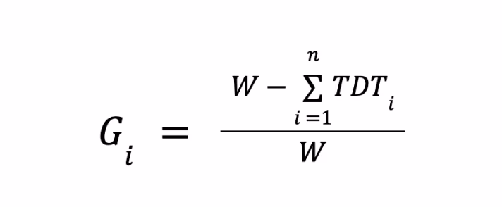
Where:

• TDTi = Training workload downtime at i’th disruption
• W = Goodput measurement time window(e.g. 24 hrs)
• n = Number of training disruptions in the window W

This captures what infra teams care about: fault detection, isolation, remediation, and restart latency. Real clusters fail in non-trivial ways at scale. The reliability literature shows that as job size grows, job-level vulnerability increases, and reliability must be engineered as a cross-layer concern rather than “just hardware.” 

Layer 2: Framework goodput – “When we fail, how much progress do we lose?”

Infra availability isn’t the full story. Even with quick restarts, training can lose progress depending on how the state is saved and restored. This is where framework goodput comes in: it measures the fraction of time not lost to checkpointing overhead and recovery waste.

Over a window (W):

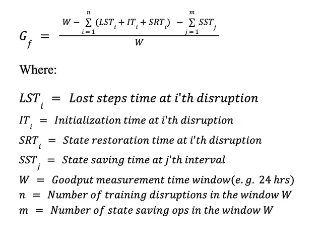
This equation makes a critical point that throughput alone hides: checkpointing is a continuous tax, while faults impose discrete penalties that often include both restart overhead and rollback waste.

Checkpointing is not “free resiliency.”

In large distributed training, checkpointing can dominate I/O and coordination overhead. Yet infrequent checkpointing increases rollback loss. The “right” checkpoint cadence is therefore a classic systems tradeoff: minimize (SST) without inflating expected (LST).

Layer 3: Model goodput – “Are we turning silicon into math efficiently?”

Even a perfectly reliable and recoverable training run can be inefficient if GPUs are poorly utilized. The standard metric here is Model FLOPs Utilization (MFU), a measure of how effectively the training program converts the peak accelerator’s capability into the FLOPs required by the model’s forward and backward passes.

A practical MFU formulation:

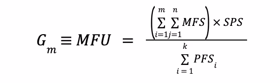
where:

• MFS = Calculated model FLOP per parameter per token per step
• m = Number of learnable model parameters
• n = Number of input tokens
• SPS = Observed steps per second
• PFSi = Theoretical peak FLOP per second on i’th GPU
• k = Number of participating GPUs

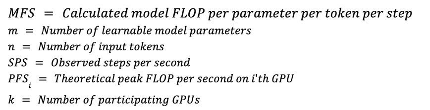
MFU is widely used to report training efficiency and is often defined as “observed model-compute rate divided by theoretical peak compute rate.”  Low MFU is usually not one “bug,” but the emergent effect of:

• Communication overhead (all-reduce/all-gather) dominating step time
• Poor parallelism configuration (TP/PP/DP/EP mismatches)
• Too-small microbatches (kernel underfill) or poor sequence/batch regime
• Memory bandwidth and activation/optimizer state pressure
• Insufficient overlap of communication with compute

This is where “program layer” choices matter: DDP vs FSDP, TP/PP choices, expert parallelism for MoE, precision (BF16/FP8), global batch size vs microbatch size, and careful scheduling of collective ops.

Combined training goodput: A stack-level efficiency metric

Once we have the three-layer-level goodputs, we can define end-to-end training efficiency as:

Training Goodput(Gt) =Gi Gf Gm

Where:

• Gi = Infra Goodput
• Gf = Framework Goodput
• Gm =  Model Goodput

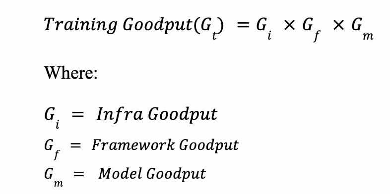
This single number ([0,1]) is useful precisely because it is stack-aware.

How to measure goodput in practice

Goodput is only as credible as its instrumentation. A practical measurement stack usually includes:

1. Establish a measurement window.

Use a fixed window (24h is common for operational reporting) and compute (Gi, Gf, Gm) over that same window to keep attribution consistent.

2. Record “productive training time” explicitly.

Log step boundaries and “training-active” state transitions. Goodput frameworks typically separate productive time from badput categories such as disruptions, restarts, checkpoint overhead, and other non-productive intervals. (Google Cloud)

3. Tie each disruption to a fault event.

Reliability work suggests measuring failures with a taxonomy and associating them with effective training time loss, which is useful both for accountability and for forecasting how failure rates scale with job size.

4. Compute MFU from steady-state training.

Exclude warmup, evaluation, long checkpoint pauses, and recovery periods when estimating MFU, unless your explicit goal is a “blended MFU.” MFU is most useful as a compute-efficiency lens during steady state.

Conclusion

LLM pretraining at scale is fundamentally a distributed systems problem wrapped around a massively parallel math problem.

Throughput (tokens/sec) is a necessary headline, but it is not a stable measure of efficiency across stacks or across time.

Goodput provides a normalized, decomposable alternative: it quantifies the fraction of potential training capacity that translates into actual training progress, and it attributes losses to the layers that can actually fix them.

As reliability research and production training platforms both underscore, scaling training is as much about reducing badput as it is about increasing peak throughput, and the most durable gains come from treating efficiency as a stack property, not a single metric.

If you’re building or operating large-scale ML systems and starting to think in terms of stack-level goodput rather than just tokens per second, the deeper work lies in how infrastructure, frameworks, and model design interact.

For continued discussions on large-scale training efficiency, resilient ML platforms, and product-driven AI infrastructure, connect with Anirban Roy on LinkedIn. You can also explore his AI interaction prototype at LLMProxy.ai

References:

1. Google Cloud: Goodput metric as measure of ML productivity (Google Cloud)
2. AWS: Checkpointless training on Amazon SageMaker HyperPod (Amazon Web Services, Inc.)
3. Kokolis et al.: Revisiting Reliability in Large-Scale Machine Learning Research Clusters (arXiv)