Holy sheet: How to create a simple to-do list with Google Sheets

Welcome to TNW Basics, a collection of tips, guides, and advice on how to easily get the most out of your gadgets, apps, and other stuff.

From your weight to your money, there’s a tracking app for everything nowadays. Sure, they can make our lives more convenient, and they give us a sense of control, but just the fact that they exist doesn’t mean we should actually use them. In fact, some are simply abusing our laziness to gather personal information for commercial purposes.

Previously, we’ve showed you how to track your stock portfolio, and how to manage your personal budget with Google Sheets. Today, we’re showing you how to manage your (personal and/or professional) to-dos by means of a simple to-do list created with… wait for it… Google Sheets! At the bottom of this article we link to the template based on the instructions we’re about to give you.

Preparing the Sheet

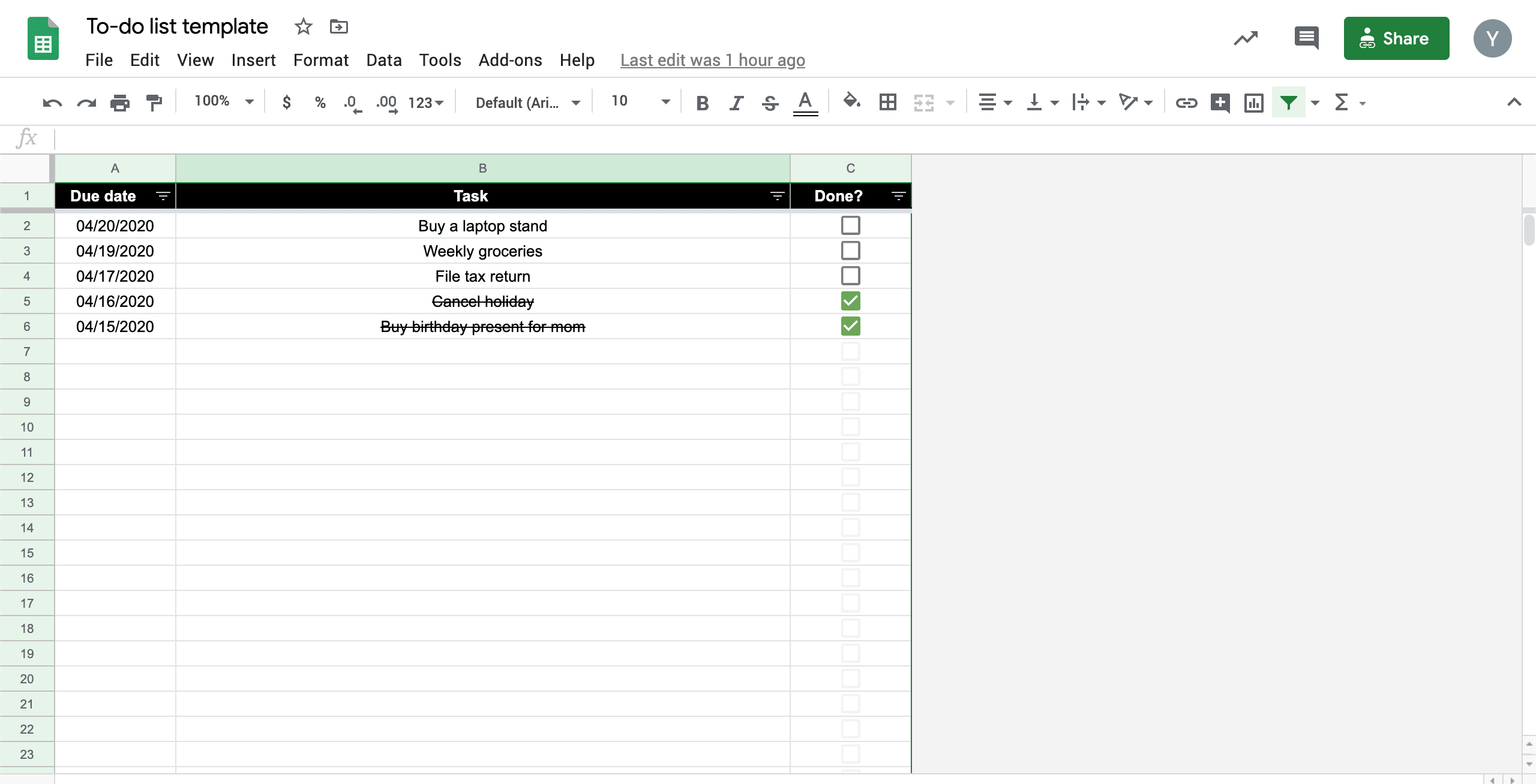
Create a new Google Sheets document. Now, add the following headers to A1, B1, and C1: ‘Due date’, ‘Task’, ‘Done?’.

To make sure the header row is fixed and doesn’t disappear no matter how long your list of to-dos becomes, select the whole first row by clicking on the ‘1’ on the left, go to menu item View, Freeze, and select 1 row.

Checkboxes and conditional formatting

We really only need two built-in features of Google Sheets to make this work. First, we need checkboxes to add a check mark to tasks that have been completed. To add a checkbox to cell C2 select C2, and go to menu item Insert, and then Insert checkbox. When you click on the checkbox in C2, the box is checked. Click one more time, and the check mark disappears again.

To make sure the whole of column C is populated with checkboxes, simply select C2, and drag the blue box at the bottom right of the cell all the way down.

Now a checkbox on itself doesn’t have much use. Ideally it is linked to a certain task, and both the task and checkbox’s styling should change based on whether the box is checked or not. For that, Google Sheets has a nifty function called Conditional formatting.

Let’s use that first to make sure a task will be strikethrough when the checkbox next to it is marked, and thus completed. Select the whole B column by clicking on the B on top of it. Now go to menu item Format, and then Conditional formatting. A sidebar tool appears.

Click + Add another rule. Change the Apply to range part to B2:B1000, to make sure the header in B1 is not influenced. Also, select Custom formula under Format cells if…. In the box below it, fill in ’=C2:C=TRUE’.

Now, under Format style select black as the text color, white as the background color, click on the strikethrough symbol, and click on the Done button. Now, whenever a checkbox is checked (TRUE), the task’s text will be strikethrough. Otherwise (not checked, thus FALSE) it will not.

Now, let’s make the check mark green so it’s a bit clearer when a task is completed. Select the C column, and go to Format, Conditional formatting, + Add another rule again. Change the range to C2:C1000, add ‘=C2:C=TRUE’ as the custom formula, select background color white, and text color a green of your choice. Click on Done. Now the check mark will be green when selected.

Finally, let’s make sure a checkbox only appears and a checkmark is only able to turn green if a task is actually filled in. Again, select the C column, Format, Conditional formatting, + Add another rule. Change the range to C2:C1000, add ‘=ISBLANK(B2:B)’ as the custom formula, select background color white, and text color the lightest gray. Click on Done.

Template

If all this still sounds too overwhelming, feel free to check out the template we made, and make a copy of the sheet (File > Make a copy) to start using it yourself.